Quantum mechanics lecture notes
The importance of quantum mechanics in chemistry is large and how there is a lot of importance on the failure of classical mechanics to describe the particles when they are at very small sizes or when describing the quantisation of energy.
Failure of classical mechanics
The first failure of classical mechanics was the description of the black body radiator. This assumed that the amount of energy a substance has is related to the wavelength of light the substance emits. This fails as it suggests that all bodies are emitting their own radiation at all times, even cool bodies will emit a blue light.
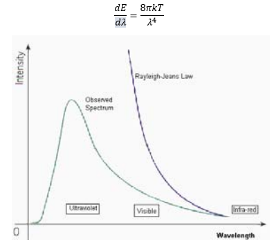
The equation here was correct at high frequencies so there was some correctness present but didn’t account for low frequency light. The mistake here was assuming the oscillator could have any frequency, this is shown by the differential in the above equation.
Planck assumed that there must be some form of quantisation in the oscillator, and assumed that the energy value would be:
Planck assumed that there must be some form of quantisation in the oscillator, and assumed that the energy value would be:

Where n is an integer, making the energy quantised. The differential equation above can then be manipulated:
This equation takes into account the frequency of the radiation in a way that at high frequencies the equation reduces to the first classical equation.
The de Broglie hypothesis-Wave particle duality and Heisenberg's uncertainty principle
Wave particle duality is important, photons of light both show particle properties in the form of discrete energy amounts but also wave like properties in diffraction. De Broglie suggested that the wavelength is associated to the momentum of the particle in the following equation:

Wave particle duality and uncertainty principle
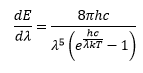
Classically a particle in space can be localised at a single position (x). In quantum mechanics the particle can be described as both a particle and a wave otherwise called a wavefunction. Now we know that a sine wave cannot be localised, it is a never ending wave. What can happen though is many sine waves can be taken into account localised at a single point forming a single point x.
The result of this is if there can be a well defined position but no knowledge of the wavelength (therefore frequency, momentum, speed).
This can be represented by Heisenberg’s uncertainty principle:
This means that neither the momentum nor position can be known exactly. This violates the underlying principles of classical mechanics. In classical mechanics if everything of the initial particle is known and assuming no outside forces act on the particle the final position can be accurately calculated.

The wavefunction
The wavefunction contains all the information of the system it describes. The momentum as a function of time of all the particles in the system this is properly written:

The Born interpretation of the wavefunction gives the probability of the particle in a given point in space. The probability that a particle is in a given volume of space dτ can be represented as:

Where Ψ* is the complex conjugate.
If a particle exists when the probability of the particle is integrated over all space then the probability of finding that particle is 1. This integration adds an normalisation factor. This is constant added to the integration. This gives us more information about Ψ If the integration is to take the value 1 and N≠0 then the wavefunction can never go to infinity.
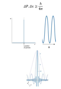
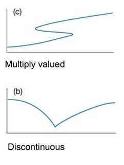
Essentially this means that the probability of finding the particle anywhere cannot be infinity meaning that the value of the integration cannot be infinity itself. This also takes into account that logically the particle cannot be in two different positions at the same time. The second and first derivatives must be well behaved, they must not be 0 or infinity. This means that the wavefunction itself must not be discontinuous anywhere. This severely limits the possibility of what can be a wavefunction or not.
If a particle exists when the probability of the particle is integrated over all space then the probability of finding that particle is 1. This integration adds an normalisation factor. This is constant added to the integration. This gives us more information about Ψ If the integration is to take the value 1 and N≠0 then the wavefunction can never go to infinity.
Essentially this means that the probability of finding the particle anywhere cannot be infinity meaning that the value of the integration cannot be infinity itself. This also takes into account that logically the particle cannot be in two different positions at the same time. The second and first derivatives must be well behaved, they must not be 0 or infinity. This means that the wavefunction itself must not be discontinuous anywhere. This severely limits the possibility of what can be a wavefunction or not.
Determining Ψ
Solving the Schrodinger equation yields vital information about the particle in question. This information can be extracted by using operators on the wavefunction.
Solving the Schrodinger equation yields vital information about the particle in question. This information can be extracted by using operators on the wavefunction.

This is a type of an equation where the same value can be extracted from each side. Ψ can be seen on both sides of the equation. This is known as an eigen equation.

This is where G^ here is an operator, f an eigenfunction and g is an eigenvalue of the operator G^
So for finding the observable of a system a different operator is used.
So for finding the observable of a system a different operator is used.
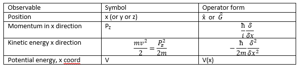
This shows how the operator changes depending on the observable needed.
The observable energy in the system is a relation between the kinetic energy and the potential energy that the particle has.
The observable energy in the system is a relation between the kinetic energy and the potential energy that the particle has.
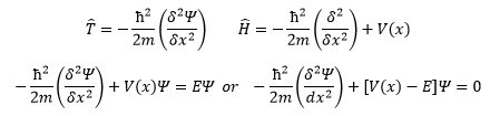
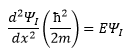
So for a free particle (all that is dealt with here) the equation is:
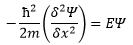
This can be re-written as:
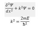
The solution of this is:
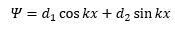
This is not helpful as the d1 and d2 cannot be quantised. The only way these are quantised are through the imposing boundary conditions such as Ψ=0 or x=0.
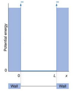
The application of this knowledge can be used in analysing the particle in a one dimensional box. This is where a particle is assumed to be in a one dimensional box with walls of infinite potential energy. This stops any tunnelling occurring and forms discrete areas that the particle cannot cross.
The particle is assumed to have no potential energy inside of the box and therefore only the kinetic energy needs to be considered.
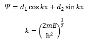
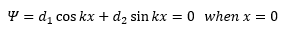
As there is no potential energy the solution to the Schrodinger equation is the same to the free particle problem assumed above.
So for the wavefunction to be continuous we know that:
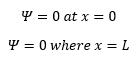
This is simple to understand as this is where the wavefunction has a nodal point. So:
Here we have just substituted 0 for the wavefunction. So when x is substituted for 0 we get:
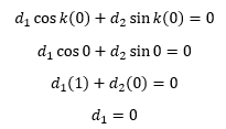
This shows how d1 equals zero so d2 can then be calculated, we already know that d1 is equal to zero so this does not need to be considered.
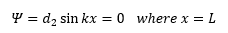
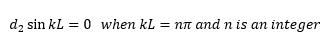
This shows how n needs to be an integer as sin π in this case needs to equal 0.
So we now have:
So we now have:

Which means we’re getting somewhere.
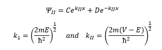
Substituting this into the original equation:
Substituting this into the original equation:
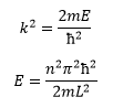
This shows that the energy must be quantised as n must be an integer for the wavefunction to hold true. So now we know what k is equal to we can go on to complete the wavefunction:
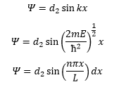
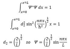
This is where d2 is the normalisation of the wavefunction. We know the wavefunction for a particle can be mapped by the following equation (link to particle in a box). This has to equal to one as the probability for the particle to be in the box is 100%.
This shows how discrete energy levels are found in a particle in a box. At larger values for n there is more energy and separations become larger at higher levels of n.
Orthogonality of wavefunctions
The orthogonality of the wavefunction is an important property of wavefunctions as wavefunctions at different energies overlap giving a total energy of zero. This severely limits the number of wavefunctions possible.
Orthogonality of wavefunctions
The orthogonality of the wavefunction is an important property of wavefunctions as wavefunctions at different energies overlap giving a total energy of zero. This severely limits the number of wavefunctions possible.
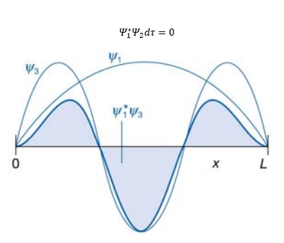
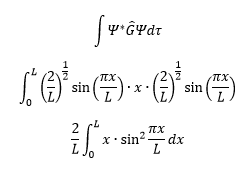
The average position can be found using the operator Ĝ, forming the following equation:
The use of particle in a box for π conjugated molecules
Using some assumptions from a particle in a box to a conjugated polymer:
· The polymer moves in 1D (it doesn’t there is no-linearality to the motion.
· Electrons move independently from one another (they don’t but very close to)
· Electrons fill orbitals according to Pauli principle.
Assuming that an electron can travel from one side of the molecule to another with little hinderance the molecule can be treated as a box.
To do this a molecule needs to be found: retinal has 12 conjugated carbon atoms and therefore 6 double bonds. It can be assumed that all of the central atoms donate 1 whole length and the end atoms ½. Using the equation for energy the following equation can be made:

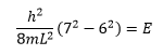
Now we have established that L=11 but what about n? It is known that 12 atoms have donated electrons so the HOMO is 6 and the LUMO is 7. This means the equation is:
Other quantised systems have the same treatment but these can be complex such as 3d boxes. This just takes into account the further dimensions. The Hamiltonian there are two cartisian coordinates around one polar coordinate.
Quantum tunneling
A free particle travelling can be represented by the following exponential form of the wavefunction:
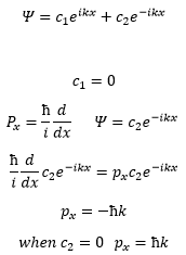
This shows how each constant represents a different x direction.
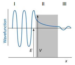
Region I
This means that in region I it is simply the free particle solution to Schrodinger’s equation.
This means that in region I it is simply the free particle solution to Schrodinger’s equation.
The general solution to this equation is:
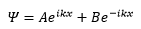
This shows how the particle can move both forwards and backwards through the space, and as there is no potential it can be represented as the wavefunction above.
Region 2
Region 2
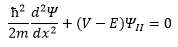
The point to be made here is when classical transition is forbidden. When E<V the solution to the equation is purely real. The absence of i means that there is no oscillation occurring in the wave. This means that a purely exponential decay forms from this point. This is now due to k becoming real due to the finite V that can be given:
This shows how the particle can still move in both directions although there is oscillation of the particle.
Region 3
Now it has to be assumed that if the particle travels through the barrier it can only be travelling in one direction which means its wavefunction becomes:
Region 3
Now it has to be assumed that if the particle travels through the barrier it can only be travelling in one direction which means its wavefunction becomes:
This is not true anywhere else as reflected particles may be present.
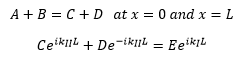
At the boundary conditions it is important that the wavefunction remains continuous. This means that:
At the boundary conditions it is important that the wavefunction remains continuous. This means that:
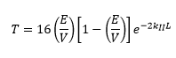
Using a lot of algebra we can see that the transmission is related to the ratio between the movement in the x direction and the wavefunction in region III.
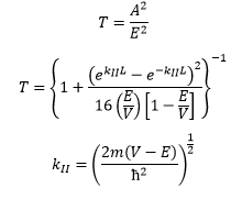
The probability of transmission is a strong function of the thickness of the barrier. It is also a strong function of the mass of the particle. A heavy particle is much less likely to pass through.
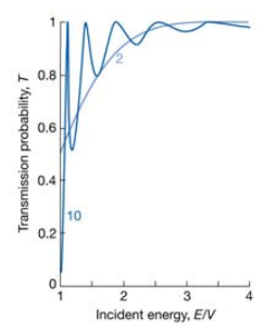
If the energy of the particle is larger than the barrier potential it is still possible for reflection to occur. Now because E>V the KII function becomes complex again so the possibility oscillates like a normal wavefunction.
If the energy of the particle is larger than the barrier potential it is still possible for reflection to occur. Now because E>V the KII function becomes complex again so the possibility oscillates like a normal wavefunction.
Scanning tunnelling microscopy
The measurement here is based on how the transmission probability depends on distance from the measurement tip.
The measurement here is based on how the transmission probability depends on distance from the measurement tip.
This measures the “tunnelling current” which has an exponential dependence on L.
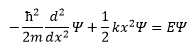
The Schroedinger equation for the SHO
The simple harmonic oscillator is a measure of the relationship between potential energy and kinetic energy.
The Schroedinger equation for the SHO
The simple harmonic oscillator is a measure of the relationship between potential energy and kinetic energy.
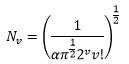
Using calculus the normalisation constant can be found:
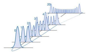
This causes there to be v number of nodes at each energy level.
The simple harmonic wavefunction then shows how the particle spends more time at the edges of the oscillator. This means at higher energy levels the particle behaves more and more classically.
The simple harmonic wavefunction then shows how the particle spends more time at the edges of the oscillator. This means at higher energy levels the particle behaves more and more classically.
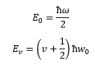
The energy levels of the simple harmonic oscillator can be represented by the following:
Born-Oppenheimer approximation (PES)
The Born-Oppenheimer approximation maps the energies of electrons as two nuclei are moved together. This gives the potential energy surface, the comparison of the separation of the nuclei and the energy of the electrons.
Solving the equation for the hydrogen atom shows that the equation can be solved. This is important as the hydrogenic atom is exactly solvable whereas any atom more complex is not so.
Heisenberg returns

This is the equation for Heisenberg we have already met, cool. This is quite simple and only gives the minimum uncertainty of the particle, in reality the uncertainty can be accurately calculated.
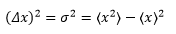
The variance needs to be calculated by:
The variance needs to be calculated by:
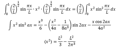
If the wavefunction is known then we can use an observable to give the mean position and therefore calculate the mean position of the particle. When it comes to finding <x2> the integral needs to be changed.
This means that the precise value of the uncertainty can be given as:
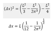
It can be found that for a 1D box the uncertainty of the particles position and momentum is given by the following equation:
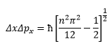
This means at lower energies there is less uncertainty.
